本次分析数据介绍：

数据为某奶茶店2018年1月-2019年6月的销售数据，共计69,659项数据，用户共计23,570名；

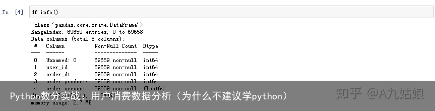
数据集共4个字段：

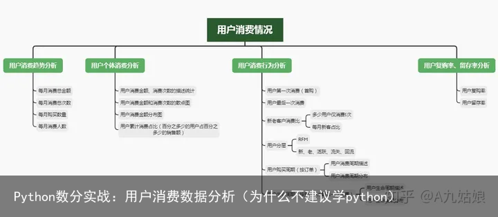
user_id: 用户idorder_id: 购买日期order_prodect: 购买产品数order_account: 购买金额

明确问题（本次数据分析目的）

用户消费趋势分析（按月）用户个体消费分析用户消费行为分析用户复购率和回购率分析

分析思路

理解数据

我们导入数据后简单看一下：

# 导入数据 df = pd.read_excel(MilkyTea_master.xlsx)

检查一下各字段类型：

数据清洗

本次抽样为全抽，不再进行选择子集；不再涉及列重命名；

1.数据类型转换

根据以上分析，我们需把用户id转化为字符串，把时间order_id转化为时间格式：

① 时间类型转换

# 时间类型转换，增加‘month’列 df[order_dt] = pd.to_datetime(df.order_dt,format=%Y%m%d) df[month] = df.order_dt.values.astype(datetime64[M])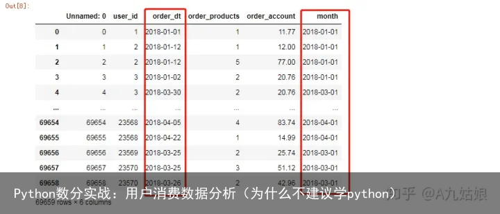

② 字符串类型转换

df[user_id] = df[user_id].apply(lambda x : str(x))

2.数据排序

# 按照“order_dt”排序 df = df.sort_values(by = order_dt,ascending =True)

3.缺失值处理

我们检查是否存在缺失值：

for i in df.columns: print(df[i].isnull().value_counts())

无需进行缺失值处理；

4.异常值处理

检查描述统计信息，查看是否存在异常

以上，我们可以发现：

大部分订单只购买了少量商品（平均值2.41），有一定极值干扰；影虎的消费金额比较稳定（平均值35.89元，中位数25.98元），有一定极值干扰；

最后，我们对index重新命名：

df = df.reset_index(drop = True)

构建模型

接下来，我们对问题进行分析：

1.用户消费趋势分析（按月）

我们按月度对用户进行分析，须将数据框按月分组：

g_month = df.groupby(month)

1）每月消费金额

# 每月消费总金额 g_month.order_account.sum()

2） 每月消费次数

# 每月消费总次数 g_month.user_id.count()

3）每月购买数量

# 每月购买数量 g_month.order_products.sum()

4）每月消费人数

# 每月消费人数 g_month.user_id.apply(lambda x : len(x.drop_duplicates()))

以上我们也可用以下方式来统一分析：

df_table = df.pivot_table(index = month, values = [order_products,order_account,user_id], aggfunc = {order_products:sum, order_account:sum, user_id:count})

我们将分析结果进行数据可视化：

sns.set_palette(summer) sns.set_style(darkgrid) f = plt.figure(figsize = (20,16)) f.add_subplot(3,1,1) g_month.order_account.sum().plot() plt.title(order_account) f.add_subplot(3,1,2) g_month.order_products.sum().plot() plt.title(order_products) f.add_subplot(3,1,3) g_month.user_id.count().plot() plt.title(user_id)

2.用户个体消费

与按月分析不同，此次需要对数据库按用户id进行分组：

1）用户消费金额、消费次数的描述统计

# 按照用户进行分组 g_user = df.groupby(user_id) # 用户消费金额、消费次数的描述统计 g_user.sum().describe() 用户平均购买奶茶7杯，中位数为3杯，说明小部分的用户购买了大量的奶茶；用户平均消费106元，中位数43元，说明小部分用户购买大量的奶茶，存在极值干扰；

2）用户消费金额和消费次数的散点图

# 用户消费金额和消费次数的散点图 g_user.sum().plot.scatter(x = order_account, y = order_products)

不是那么明显，我们选择购买金额<6000的数据集进行分析（去除极值）：

# 用户消费金额和消费次数的散点图 g_user.sum().query(order_account < 6000).plot.scatter(x = order_account, y = order_products)

3）用户消费金额分布图

# 用户消费金额分布图 g_user.sum().order_account.plot.hist(bins = 20)

可知，用户消费金额大部分呈集中趋势，小部分异常值干扰了判断；

我们可以运用切比雪夫定理：‘所有数据中，至少有24/25（或96%)的数据位于平均数5个标准差范围内’，故，我们用7+16.98*5 ≈100 来排出异常值：

g_user.sum().query(order_account < 100).order_account.plot.hist(bins = 20)

4）用户累计消费占比（百分之多少的用户占百分之多少的销售额）

# 用户累计消费占比（百分之多少的用户占百分之多少的销售额） g_user.sum().sort_values(order_account).apply(lambda x : x.cumsum()/ x.sum()).reset_index().order_account.plot()

按用户消费金额升序排列，上图可知，60%的销售金额是被前5000名（近20%）的人贡献；而50%的用户仅贡献了15%的销售额；

3.用户消费行为分析

同样，我们依旧按用户分组进行分析：

1）用户第一次消费（首购）

# 用户第一次消费（首购） g_user.min().order_dt.value_counts().plot()

用户首购分布：集中在前3月；在2月中旬期间，波动较剧烈；

2）用户最后一次消费

# 用户最后一次消费 g_user.max().order_dt.value_counts().plot()

用户最后一次购买时间分布较广，大部分最后一次购买集中在前3个月，说明可能存在很多用户购买了一次没有再复购；随着时间递增，最后一次购买的用户数量也在上升，消费呈流失上升状态；

3）新老客户消费比

① 多少用户仅消费1次

# 多少用户仅消费1次 user_life = g_user.order_dt.agg([min,max]) (user_life[min] == user_life[max]).value_counts() # 可视化（饼图） plt.pie((user_life[min] == user_life[max]).value_counts(normalize = True), autopct=%.2f%%, labels = (user_life[min] == user_life[max]).value_counts().index)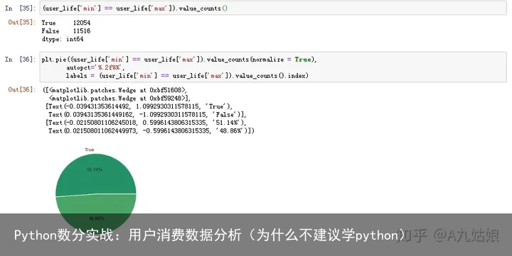

我们发现，超过一半用户仅消费一次；

② 每月新客占比

# 每月新客占比 g_user.min().month.value_counts() / g_month.user_id.apply(lambda x : len(x.drop_duplicates()))

我们发现，首月消费新客占比100%，第二、三月逐渐新客数量占比减少，第四月后无新客；

4）用户分层

① RFM用户分层

这里需要补充一下RFM分析：

RFM是3个指标的缩写，最近一次消费时间间隔（Recency），消费频率（Frequency），消费金额（Monetary）。通过这3个指标对用户分类。最近一次消费时间间隔（R），上一次消费离得越近，也就是R的值越小，用户价值越高；消费频率（F），购买频率越高，也就是F的值越大，用户价值越高；消费金额（M），消费金额越高，也就是M的值越大，用户价值越高；

所以，我们根据以上内容，对数据集根据order_products,order_account,order_dt进行数据透视：

# RFM用户分层 rfm = df.pivot_table(index = user_id, values = [order_products,order_account,order_dt], aggfunc= {order_products:sum, order_account:sum, order_dt:max})

我们对最后一次消费时间计时间间隔，并对透视结果列重命名：

rfm[R] = (rfm.order_dt.max() - rfm.order_dt) / np.timedelta64(1,D) rfm.rename(columns={order_products:F,order_account:M},inplace = True)

建立RFM模型：

def rfm_func(x): level = x.apply(lambda x:1 if x > 0 else 0) label = level.R +level.F + level.M d = { 111:重要价值客户, 011:重要保持客户, 101:重要发展客户, 001:重要挽留客户, 110:一般价值客户, 010:一般保持客户, 100:一般发展客户, 000:一般挽留客户 } result = d[label] return result rfm[label] = rfm[[R,F,M]].apply(lambda x : x - x.mean()).apply(rfm_func,axis=1)

接着，我们对‘label’列分组求和：

rfm.groupby(label).sum()

我们也可以分组后计数：

rfm.groupby(label).count()

从RFM分层可知，大部分的用户是一般挽留客户，重要价值客户和重要保持客户合计约占20%；

我们进行可视化：

rfm.loc[rfm.label == 重要价值客户,color] = g rfm.loc[rfm.label != 重要价值客户,color] = r rfm.plot.scatter(F,R,c = rfm.color)

② 用户生命周期-新、老、活跃、回流、流失

# 用户生命周期-新、老、活跃、回流、流失 pivoted_counts = df.pivot_table(index = user_id, columns= month, values= order_dt, aggfunc= count).fillna(0)

需要对结果进行简化，如果购买次数大于0（大于等于1），有购买为1，无购买为0：

# 进行简化 df_purchase = pivoted_counts.applymap(lambda x : 1 if x>0 else 0)

根据本月是否消费、前期是否消费、上月是否消费等多层维度，将用户划分为未注册、新注册、活跃、不活跃、回流、流失；

def active_statu(data): status = [] for i in range(18): # 当月未消费 if data[i] == 0: if len(status) > 0: if status[i-1] == unreg: status.append(unreg) else: status.append(unactive) else: status.append(unreg) # 当月有消费 else: if len(status) == 0: status.append(new) else: if status[i-1] == unactive: status.append(return) elif status[i-1] == unreg: status.append(new) else: status.append(active) return status purshase_stats = df_purchase.apply(active_statu,axis=1) purshase_stats = pd.DataFrame(purshase_stats)[0].apply(pd.Series) purshase_stats.columns = pivoted_counts.columns

把‘unreg’用NAN替换，并对每月的用户状态进行统计：

purshase_stats_ct = purshase_stats.replace(unreg,np.NAN).apply(lambda x : pd.value_counts(x))# 转置 purshase_stats_ct.fillna(0).T

可视化：

purshase_stats_ct.fillna(0).T.plot.area()

可以逐行计算百分比：

# 可以逐行计算百分比 purshase_stats_ct.fillna(0).T.apply(lambda x : x/x.sum(),axis = 1) purshase_stats_ct.fillna(0).T.apply(lambda x : x/x.sum(),axis = 1).plot.area()

5）用户购买周期（按订单）

① 用户订单周期

# 用户订单周期 order_diff = g_user.apply(lambda x: x.order_dt - x.order_dt.shift())

查看描述统计：

② 用户订单分布

(order_diff/np.timedelta64(1,D)).hist(bins=20)订单周期呈指数分布用户平均购买周期是68天绝大部分用户购买周期都超过100天

6）用户生命周期（按第一次&最后一次消费）

我们查看用生命周期（第一次&最后一次）描述统计：

(user_life[max] - user_life[min]).describe()((user_life[max] - user_life[min])/np.timedelta64(1,D)).hist(bins = 40)用户生命周期受只购买一次的用户影响较大用户平均消费时间差134天，中位数仅0天

4.用户复购率和留存率

1）复购率

自然月内，购买多次的用户占比：

我们根据上述的对用户按月统计购买量pivoted_counts来分析：

如果当月购买了1次以上（大于1），则为1，存在复购；若购买了1次，为0；当月购买了0次，则为NAN；

purchase_r = pivoted_counts.applymap(lambda x : 1 if x > 1 else np.NAN if x == 0 else 0 )

求和，为当月复购的人数；计数，为当月购买人数：

(purchase_r.sum() / purchase_r.count()).plot(figsize = (10,4))

复购率稳定在20%左右，前三月因为有大量的新用户涌入，而这批用户只购买了一次，所以导致复购率低；

2）回购率（留存率）

曾经购买过的用户某一时间内再次购买的占比：

定义函数，如果当月购买，下月也购买为1；如果当月购买下月未购买，为0；如果当月未购买，则为NAN；

def purchase_back(data): status = [] for i in range(17): if data[i] ==1: if data[i+1] == 1 : status.append(1) if data[i+1] == 0 : status.append(0) else: status.append(np.NAN) status.append(np.NAN) return status purchase_b = df_purchase.apply(purchase_back,axis=1) purchase_b = pd.DataFrame(purchase_b)[0].apply(pd.Series) purchase_b.columns = pivoted_counts.columns

回购率 = 次月再次购买/本月购买人数

(purchase_b.sum()/purchase_b.count()).plot(figsize = (10,4))

分析结论

用户增长阶段仅在前三月，后期消费均为老客户；消费用户群体较为固定；超过50%的用户仅在前三月消费了一次，后期长期处于不活跃状态；用户消费呈流失上升状态；60%的销售金额是被前5000名（近20%）的人贡献。

以上就是我们利用Python对用户消费情况、用户分层、用户生命周期及复购率、回购率简单的分析。